
FRED Overview
Contents
FRED Overview#
In order to programatically request data from FRED, you first need to first request an api key from the FRED website. After you have done so, you’ll have the ability to request data from FRED via python. The python package I have always used is fredapi. There isn’t any special reason why I chose this package over the other ones I have seen, but it was the first one I encountered a long time ago and it hasn’t failed me yet, so I have felt no urge to change.
Establishing a FRED object#
Step one when using FRED is to import the package and establish a master “fred” object. The fred object is the primary work horse and will be doing most of the heavy lifting.
from fredapi import Fred

# Load in api from config file
with open('secrets.yml') as f:
    secrets = yaml.safe_load(f)


fred = Fred(api_key=secrets['fred_api_key'])
Requesting Data#
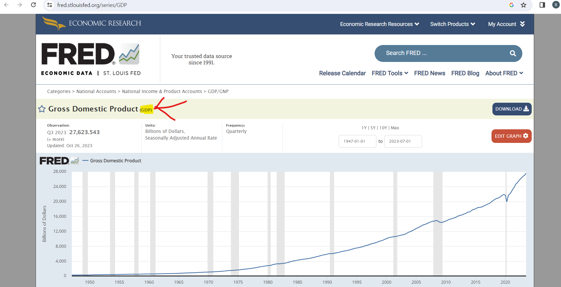
Now, let’s say we would like to see the US Nominal GDP growth over time. The steps to doing this are:
Find the data on FRED (Google tends to work better than directly searching in fred)
My search: “fred us nominal gdp”
Verify this is the data you want.
Copy the series ID: found in the url or right after the title of the series.
Call the ‘get_series’ method on the fred object and pass the series ID as an argument:
Note: There are other arguments you can pass to the ‘get_series’ method, such as start and end dates, but I tend to just request all of the data and do any filtering as-needed later on.
# Pull Data:
us_nominal_gdp = fred.get_series('GDP')

# For some reason, FRED returns the values in 1946 as nan, so drop those:
us_nominal_gdp = us_nominal_gdp.dropna()

# Also, I think the data prints prettier in the notebook if it is converted to a DataFrame:
us_nominal_gdp = pd.DataFrame(data=us_nominal_gdp, columns=['GDP'])
us_nominal_gdp
| GDP | |
|---|---|
| 1947-01-01 | 243.164 |
| 1947-04-01 | 245.968 |
| 1947-07-01 | 249.585 |
| 1947-10-01 | 259.745 |
| 1948-01-01 | 265.742 |
| ... | ... |
| 2022-07-01 | 25994.639 |
| 2022-10-01 | 26408.405 |
| 2023-01-01 | 26813.601 |
| 2023-04-01 | 27063.012 |
| 2023-07-01 | 27644.463 |
307 rows × 1 columns
That’s basically all there is to it!
Helpful Functions#
There are a few tasks that I tend to do frequently when working with FRED data after pulling it from the api. Because of that, I created a few helper functions that I use as a wrapper around the api. These are what I primarily interact with. Some of the “enchancements” that I like:
Converting from series to a dataframe.
Providing a better name for the data, rather than the FRED series id.
Send in an iterable of ids to request data in bulk.
Merge the data together
So these are the functions I made:
def get_fred_data_series(series_id: str, name: Optional[str] = None) -> pd.DataFrame:
    '''This function pulls data from FRED and returns it as a DataFrame, if you input a name, it will use that as the
      column name, otherwise it will use the series_id as the column name. '''

    data_name = name if name is not None else series_id
    df = fred.get_series(series_id).to_frame()
    df.columns = [data_name]
    df.index.name = "date"
    return df

def get_fred_data(series_ids: Union[List[str],str], names: Optional[Union[List[str],str]] = None,merge_data:bool=True) -> Union[pd.DataFrame,dict]:

    # If the input was a string, we can just call the get_fred_data_series function once right now and return the result
    if isinstance(series_ids, str):
        return get_fred_data_series(series_ids, names)


    names = names if names is not None else series_ids
    ids_and_names = zip(series_ids, names)
    # Now pull the data
    all_data = [get_fred_data_series(series_id, name) for series_id, name in ids_and_names]

    if merge_data:
        result = pd.concat(all_data, axis=1,join='outer')
    else:
        result = dict(zip(series_ids,all_data))

    return result
To get a feel for it, and make sure it works, here are a few tests. First, single data series:
get_fred_data('GDP').tail()
| GDP | |
|---|---|
| date | |
| 2022-07-01 | 25994.639 |
| 2022-10-01 | 26408.405 |
| 2023-01-01 | 26813.601 |
| 2023-04-01 | 27063.012 |
| 2023-07-01 | 27644.463 |
Now, try sending in multiple series ids that we want to combine - GDP, Real GDP, and cpi:
DATA_TO_REQUEST = ['GDP','GDPC1','CPIAUCSL']
DATA_NAMES = ['GDP','Real GDP','cpi']
data_df = get_fred_data(DATA_TO_REQUEST, DATA_NAMES)
data_df.tail()
| GDP | Real GDP | cpi | |
|---|---|---|---|
| date | |||
| 2023-06-01 | NaN | NaN | 303.841 |
| 2023-07-01 | 27644.463 | 22506.365 | 304.348 |
| 2023-08-01 | NaN | NaN | 306.269 |
| 2023-09-01 | NaN | NaN | 307.481 |
| 2023-10-01 | NaN | NaN | 307.619 |
Beautiful, now test how it looks if we don’t want to combine the data.
DATA_TO_REQUEST = ['GDP','GDPC1','CPIAUCSL']
DATA_NAMES = ['GDP','Real GDP','cpi']
# Below function will return a dictionary of DataFrames
data_dict = get_fred_data(DATA_TO_REQUEST, DATA_NAMES,merge_data=False)

# Show me the inflation data:
data_dict['CPIAUCSL']
| cpi | |
|---|---|
| date | |
| 1947-01-01 | 21.480 |
| 1947-02-01 | 21.620 |
| 1947-03-01 | 22.000 |
| 1947-04-01 | 22.000 |
| 1947-05-01 | 21.950 |
| ... | ... |
| 2023-06-01 | 303.841 |
| 2023-07-01 | 304.348 |
| 2023-08-01 | 306.269 |
| 2023-09-01 | 307.481 |
| 2023-10-01 | 307.619 |
922 rows × 1 columns
Examples#
Finally, here are a few more examples of seeing how the data might be used in action to create some informative plots.
US GDP Growth#
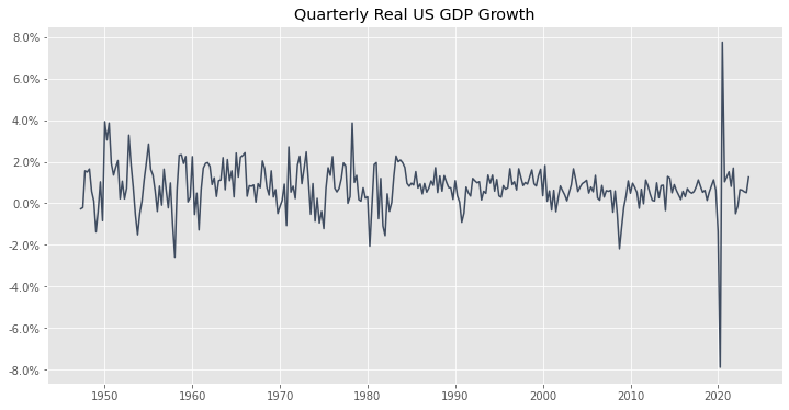
We sort of already saw this above, but just to be thorough, let’s examine the quarterly growth rate of Real GDP in the US for as far back as FRED will let us look.
# Request the data and verify that it looks ok:
DATA_TO_REQUEST = ['GDPC1']
gdp_df = get_fred_data(DATA_TO_REQUEST)

# Calculate the Quarterly Growth Rate:
gdp_df['quarterly_growth'] = gdp_df['GDPC1'].pct_change()

# Drop NaNs that were introducted by the pct_change function (We also need to drop those NANs from 1926.)
gdp_df = gdp_df.dropna()

gdp_df.tail()
| GDPC1 | quarterly_growth | |
|---|---|---|
| date | ||
| 2022-07-01 | 21851.134 | 0.006586 |
| 2022-10-01 | 21989.981 | 0.006354 |
| 2023-01-01 | 22112.329 | 0.005564 |
| 2023-04-01 | 22225.350 | 0.005111 |
| 2023-07-01 | 22506.365 | 0.012644 |
Looks good, so let’s go ahead and plot the data, for good measure.
fig, ax = plt.subplots(figsize=(12,6))
ax.plot(gdp_df['quarterly_growth'])
ax.yaxis.set_major_formatter(FuncFormatter(percentage_formatter)) # Format the y-axis as percentages
ax.set_title('Quarterly Real US GDP Growth');
Display some summary stats as well:
gdp_df['quarterly_growth'].describe().to_frame()
| quarterly_growth | |
|---|---|
| count | 306.000000 |
| mean | 0.007717 |
| std | 0.011260 |
| min | -0.078910 |
| 25% | 0.003105 |
| 50% | 0.007721 |
| 75% | 0.012623 |
| max | 0.077592 |
What quarters had the lowest and highest GDP changes?
min_growth = gdp_df['quarterly_growth'].min()
max_growth = gdp_df['quarterly_growth'].max()


min_max_results_df = gdp_df[(gdp_df['quarterly_growth'] == min_growth) | (gdp_df['quarterly_growth'] == max_growth)].copy()

# Add a column to label the min and max values... Just to make it super easy on the eyes:
min_max_results_df.loc[min_max_results_df['quarterly_growth'] == min_growth, 'Label'] = 'Minimum'
min_max_results_df.loc[min_max_results_df['quarterly_growth'] == max_growth, 'Label'] = 'Maximum'

min_max_results_df
| GDPC1 | quarterly_growth | Label | |
|---|---|---|---|
| date | |||
| 2020-04-01 | 19034.830 | -0.078910 | Minimum |
| 2020-07-01 | 20511.785 | 0.077592 | Maximum |
The minimum and maximum GDP growth rates were when the economy was first entering and exiting COVID. Makes sense.
Inflation#
Inflation is another hot topic right now. Something interesting to note is that when most news articles or commentators are discussing inflation, they are usually referencing the CPI index. But the Federal Reserve Board of Governors has stated that they use the PCE index as their preferred gauge of inflation. That feels a little wierd, why the inconsistency? For now, I’ll ignore the why behind the discrepancy, and instead use FRED to show that they are basically the same thing:
INFLATION_SERIES = ['CPIAUCSL','PCEPI']
DATA_NAMES = ['CPI','PCE']
inflation_df = get_fred_data(INFLATION_SERIES, DATA_NAMES)

# YoY Inflation Rate:
inflation_df['CPI_YoY'] = inflation_df['CPI'].pct_change(12)
inflation_df['PCE_YoY'] = inflation_df['PCE'].pct_change(12)


# Drop nas:
inflation_df = inflation_df.dropna()
inflation_df
| CPI | PCE | CPI_YoY | PCE_YoY | |
|---|---|---|---|---|
| date | ||||
| 1960-01-01 | 29.370 | 15.421 | 0.012410 | 0.016948 |
| 1960-02-01 | 29.410 | 15.437 | 0.014138 | 0.016997 |
| 1960-03-01 | 29.410 | 15.446 | 0.015188 | 0.016920 |
| 1960-04-01 | 29.540 | 15.502 | 0.019324 | 0.018595 |
| 1960-05-01 | 29.570 | 15.518 | 0.018251 | 0.019111 |
| ... | ... | ... | ... | ... |
| 2023-06-01 | 303.841 | 120.221 | 0.030920 | 0.031984 |
| 2023-07-01 | 304.348 | 120.438 | 0.032991 | 0.033705 |
| 2023-08-01 | 306.269 | 120.877 | 0.037075 | 0.034109 |
| 2023-09-01 | 307.481 | 121.325 | 0.036899 | 0.034190 |
| 2023-10-01 | 307.619 | 121.385 | 0.032324 | 0.030066 |
766 rows × 4 columns
fig, ax = plt.subplots(figsize=(12,6))
ax.plot(inflation_df['CPI_YoY'], label='CPI ')
ax.plot(inflation_df['PCE_YoY'], label='PCE')
# Format the y axis as a percent:
ax.yaxis.set_major_formatter(FuncFormatter(percentage_formatter))
ax.set_title('CPI vs PCE')
ax.legend();
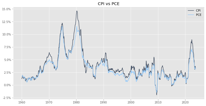
So yea, they track each other pretty closely! To be precise and quantitive about exactly how close “pretty close” is, we can calculate the correlation between the rates of inflation using each index:
correlation = inflation_df['CPI_YoY'].corr(inflation_df['PCE_YoY'])
print(f"The correlation between CPI and PCE is: {correlation:.2f}")
The correlation between CPI and PCE is: 0.98
VIX#
vix_df = get_fred_data('VIXCLS', 'VIX')
# For some reason, there are many missing values in the VIX data, so we will interpolate those:
vix_df['VIX'] = vix_df['VIX'].interpolate()
# Rolling 1 month average:
vix_df['VIX_1M'] = vix_df['VIX'].rolling(22).mean()
# Rolling 3 month average:
vix_df['VIX_3M'] = vix_df['VIX'].rolling(365).mean()
# Entire time period average:
vix_df['VIX_AVG'] = vix_df['VIX'].mean()
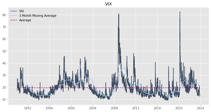
# Plot the data: (Not plotting the 1-Month because it follows the actualy number pretty close and the graph is too busy)
fig, ax = plt.subplots(figsize=(12,6))
ax.plot(vix_df['VIX'], label='VIX')
ax.plot(vix_df['VIX_3M'], label='3 Month Moving Average')
ax.plot(vix_df['VIX_AVG'], label='Average', linestyle='--')
ax.set_title('VIX')
ax.legend();
# Display the data:
vix_df
| VIX | VIX_1M | VIX_3M | VIX_AVG | |
|---|---|---|---|---|
| date | ||||
| 1990-01-02 | 17.24 | NaN | NaN | 19.591738 |
| 1990-01-03 | 18.19 | NaN | NaN | 19.591738 |
| 1990-01-04 | 19.22 | NaN | NaN | 19.591738 |
| 1990-01-05 | 20.11 | NaN | NaN | 19.591738 |
| 1990-01-08 | 20.26 | NaN | NaN | 19.591738 |
| ... | ... | ... | ... | ... |
| 2023-11-24 | 12.46 | 15.317273 | 19.990603 | 19.591738 |
| 2023-11-27 | 12.69 | 14.954091 | 19.949945 | 19.591738 |
| 2023-11-28 | 12.69 | 14.564091 | 19.909260 | 19.591738 |
| 2023-11-29 | 12.98 | 14.256364 | 19.871589 | 19.591738 |
| 2023-11-30 | 12.92 | 14.019091 | 19.835534 | 19.591738 |
8848 rows × 4 columns
# Show some basic summary statistics:
vix_df['VIX'].describe().to_frame()
| VIX | |
|---|---|
| count | 8848.000000 |
| mean | 19.591738 |
| std | 7.893034 |
| min | 9.140000 |
| 25% | 13.900000 |
| 50% | 17.790000 |
| 75% | 23.010000 |
| max | 82.690000 |
Future To DO?#
Show how to get unrevised data